Fourier analysis - Sines and Integrals (part 2)

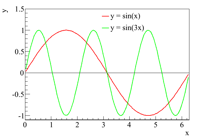
In the last post, I attempted to remind the reader of the definition of a sine curve. I particularly wanted to highlight that the sine function is the mathematical representation of a wave, and since waves are representations of musical notes, a sine curve is also a mathematical representation of a musical note. Those who are familiar with music (or perhaps with my post on the guitar back in November) will be aware that different musical notes are simply waves with different frequencies. That is easily related to the sine curve by multiplying the variable by some number. For example, I've been showing plots of just the basic sine function, y = sin(x) or y = sin(θ). If, however, I decided to plot y = sin(3x), then all of a sudden the frequency of the wave would be tripled, as in this figure:

It is pretty clear that during the time it takes the standard sine function (the red curve) to undergo a full oscillation, the higher frequency curve (the green curve) represented by y = sin(3x) has undergone three full oscillations. Thus, I can represent any of the musical notes using the sine function, simply by changing the multiplication factor. This is essentially what I did in the graphical representations from the November post, by just adding different functions together to produce the sounds I wanted.

We are now ready to talk about the two fundamental keys to Fourier analysis. The first is that any periodic signal can be obtained simply by adding sine curves of different frequencies. To illustrate this, I'm going to draw on everyone's friend, Wikipedia, which has a great entry on Fourier analysis and Fourier series (which does raise the question, "why am I bothering to do this when so many other people have already done it before?" but then this is my blog and I can do it again if I want to. In general, for those who are interested, Wikipedia is really good at mathematical concepts, and I use it as a reference all the time). In the Fourier series article, the unnamed Wikipedia author is exactly illustrating the point I'm making here, that any periodic function can be expressed as the sum of sine curves with different frequencies.

The first example is the square wave. This is a wave that alternates between two values, for example either 1 or -1, so that it looks like a box. The sine function is very smooth, so it may seem hard to believe that you can get a square wave from sines. But, as in the following picture, it doesn't take very many iterations before the sines do a pretty good job at imitating the square wave:


A second example, featuring our favorite gimmick animation, is the the sawtooth wave. Assuming I get this to work right, the animation should show a sawtooth wave along with the sum of sines as each additional sine is added to the total. As with the square wave, the approximation gets pretty good without too many steps:


From here, it should be easy to imagine creating the shapes from my guitar post simply by adding different notes together. The second key will be the subject of the next post.

Fourier analysis - Sines and integrals

In case anyone is still reading this, now that it is being updated so sporadically, I'm finally managing another post on Fourier analysis. In this post, I'll try to set up a little bit of the math behind the theory. To do so, I'm going to first remind everyone about the sine function, which I wrote about when talking about the Double Slit Experiment. In that post, I said that the sine function was a mathematical representation of a wave. Here is a plot of y = sin(θ):
Now, that looks an awful lot like the sound waves I was looking at with my guitar back in November. Because they are the same. In fact, when I wanted to depict the sound waves graphically, I used the sine and its partner, the cosine to do it. Going back to the post on the double slit experiment, I believed I compared these functions to a part of speech; by using them, I can now describe a whole host of different phenomena that were previously inaccessible. Including sound waves.

Next, I want to talk about integrals. My mother never took calculus and says she has no idea what an integral is, which means I'm going to try to give a brief introduction (without going into details, alas). The first thing I was taught about integrals is that they represent the "area under the curve," and I think that's really all we need to know about them. If I draw a curve on a coordinate system, for example, like the sine curve above, then the integral is the area between the curve and the x-axis. Therefore, we need to know one other thing to define it, and that is the range of the integral. For example, I am going to zoom in slightly on that sine curve, and then I'll take the integral from x = 0.5 to x = 2.5, which is just the area below the curve between those limits, or the region shaded green.



Now, things can get a bit trickier conceptually when the curve crosses the x-axis and becomes negative-valued. In this case, the integral is still the area under the curve, except that it is now negative. This is represented by the yellow shading.



Finally, if you look carefully, you'll notice that the sine function appears to be symmetric. This will be really important for Fourier analysis. If you integrate the sign function over an entire period, the positive part and the negative part cancel each other out, and we're left with a total integral of 0.



I want to make two final comments about integrals. The key to calculus is finding out that you can generally solve for these areas if you know the functional form of the curve (in this case, for example, we know the curve is a sine curve, so I could write down the function representing the area from calculus). And because I know this is the kind of thing that might interest my mom, in math, we represent an integral with a symbol that looks a little bit like an "S". For example, the integral of sin(x) is written like this:

$\int sin(x)dx$

The "dx" is there partly to let the reader know that the integral is being performed over the x variable.

Carl Wieman and learning science

This will be the second non-Fourier post I will write, and again I apologize. Who knew that writing a thesis and applying for jobs was so demanding? The subject of this post is learning and teaching science. This week, we had Nobel Laureate Carl Wieman visiting Yale, and he gave two great talks on research people have done on how students actually learn science. Professor Wieman has been applying scientific methods to scientific learning for some time now, and among other things, he writes a blog about it.

One of the more interesting conclusions is that the standard lecture format of undergraduate courses is poorly matched to the way people actually learn and retain scientific understanding - in fact, often students come out of these classes thinking more like a "novice" scientist than when they started. By novice, I mean the following: there are certain ways that an expert in a scientific field thinks about that field that are very different from the way a novice thinks about that field. For example, a novice believes that scientific content consists of isolated pieces of information that have been handed down by some authority and require memorization. An expert believes that scientific content consists of a coherent structure of concepts that build on each other, being accurate descriptions of nature and established by experiment. Sad to say, but students coming out of intro science classes are even more likely to believe that science is bits of memorization based on nothing more than faith, as opposed to a coherent argument based on reality.

These results resonated with me, because in this blog, I've tried to emphasize how one builds to a conclusion (like "dark matter exists") from a variety of physical observations and theories (like the 20 posts that followed my original three). I'm sure that sometimes (often?) I fail in communicating this key point about the way I look at physics, but that is ultimately the goal of this blog. And when I start writing it again regularly, I'll try not to forget that.

Finally, Wieman and his group have developed a series of simulations for students to play with that really demonstrate key concepts of physics. One example that caught my eye is something that I tried to explain in a post a few months ago, the photoelectric effect. If a reader really wants to understand what I was trying to say in that post, I highly recommend trying out Wieman's simulation, located here. Especially you, mom (although she's currently in India right now, and therefore not reading this blog at all. By the time she gets back, I'll be writing more regularly...)

The CDMS result

Merry Christmas, everyone. I know I promised more on Fourier analysis, and I'll get to it, but I want to take a slight detour to mention some exciting results announced last week by the Cryogenic Dark Matter Search (CDMS), a dark matter experiment based on a different technology than my own. For the last decade, CDMS has been the leading experiment in the field, and their new result is no different. A week ago, CDMS released the results of their most recent analysis, and lo and behold! they had some events. This is exciting.

Before going forward, I'll just mention the methodology at work here. With some notable exceptions (like DAMA, for example), most dark matter experiments work by pushing down the backgrounds as much as possible to reveal the dark matter signal that may or may not be there. Therefore, the majority of work goes into understanding exactly how much background might be left over, with the goal to have "zero" background during the time the experiment is looking for WIMPs. It is generally impossible to have "zero" background - what is possible is a very small fractional expectation of a background. For example, CDMS expected 0.6 background events in their data set. What that means is they studied all possible sources of background using calibration sources and simulations and estimated that in the amount of time they looked for dark matter, on average they would see 0.6 background events.

When they looked at their data, they found 2 events. One can calculate the probability of having 2 background events given an expectation of 0.6, and CDMS has done this; they determined that there was about a 25% chance that the two events could be a fluctuation on the background, leaving a 75% chance that the 2 events were something new, like a dark matter interaction. This is not enough significance to claim a discovery (most physics experiments require a measurement with over a 99.999% chance of being something new before a discovery can be claimed), but it is exciting. Up until now, most experiments have never claimed to see something over background, so these results are a sign that there might actually be something to the last five years of my life. Of course, it's always possible CDMS underestimated their backgrounds.

As mentioned in the NYTimes article, we'll now wait with bated breath for the results from XENON100 in Italy, which should be the next experiment to get results. If the 2 events in the CDMS data are real dark matter events, XENON100 should be able to find out. And then my experiment should follow that up with our own search in a year or two. It's a good time to be involved in dark matter - who knows, maybe we'll figure out one of the biggest mysteries in physics from the last 70 years before the next presidential election.

Fourier analysis 2 - More complicated sound waves

I imagine the discussion in the previous entry seems pretty boring. It was really easy to tell apart the A note from the white noise, both by sound and by looking at the graphical representation. Things get more complicated however when we add more notes to make a chord or a complicated piece of music. For example, a simple A chord consists of three notes - A, C# and E. The nearest C# to the standard A has a frequency of 523.25 Hz while the nearest E has a frequency of 659.26. Here's what that sounds like on my guitar (it's sort of fun posting videos of my guitar online), followed by the graphical image:




One can still see the oscillatory behavior, but things aren't quite as clean as they were when I was plotting just the simple A note.

Now, what happens if I play a full A chord by adding A notes from the next two octaves up and another C# as well?



You can still see a few clear features, but overall it doesn't look nearly as obvious that this is an actual chord. In reality, no sound wave is perfectly free of noise either. We are all familiar with static in our speakers and acoustic reflections tend to add noise to the wave as well. In general, external sources of static add white noise on top of the underlying wave. In such a situation, it can be impossible to see the wave underneath the noise just by eye.

This is where Fourier analysis comes in. Fourier analysis is a mathematical method that can decompose signals like the ones shown in the various pictures into their constituent waves. By Fourier analyzing a pulse, we can find out how much of each pulse is contributed by a wave of a particular frequency. For example, returning to the simple A note, the entire pulse is a wave of 440 Hz. Therefore, the Fourier transform of that plot should provide us with a peak at 440 Hz, and nothing else. Here's what the Fourier transform of the A note looks like:


The Fourier transform has picked out the signal at 440 Hz, and shown that it is the only component there. What about white noise, where there is no dominant frequency component? Fourier analysis can find that as well.



And finally, where Fourier analysis really shines is when the signal is so complicated that one couldn't possibly tell apart all its constituents by eye. For example, look at the Fourier decomposition of the full A chord - all of the 6 notes are clearly broken out in the decomposition and we can understand exactly what went into the making of that sound.


I have one last example, just because I think this is so cool. I made a signal of 12 semi-random frequencies, with a little white noise added. The first plot is what they look like in the time domain (i.e. when you plot the amplitude of the sound as a function of time). There's no real pattern there that I can see. But when I plot the Fourier transform, there they all are. It's like magic. But it's not, it's just math, and I'll try to explain it qualitatively in the next post.

Fourier analysis 1 - Sound waves

First, I need to apologize for the lack of activity on this blog, and regretfully state that the relative dearth of new posts will likely continue for another few months. I'm at the point of my career when I try to graduate and get a job for next year, and between these two activities I don't have much time for posting to this blog. I do plan on continuing it, but it will of necessity be sporadic for a few more months.

Now that that is out of the way, I want to discuss Fourier analysis, which I mentioned at the end of the last post (over two months ago). One theme that may have come through to someone reading this blog since the beginning is the ubiquity of "waves" in physics. When discussing the Doppler effect back in March, I used sound as an example (the police siren) before moving to light. I want to do the same thing now. Sound is a pressure wave that moves through the air and is interpreted by our ears. Just as the color of light is determined by its frequency, the pitch of sound is also determined by the frequency of the sound wave. People who play music will be very familiar with this - the root A note, for example, is a sound wave with a frequency of 440 Hz (if I haven't used this unit before, a Hz is just inverse seconds. So 440 Hz means that the wave oscillates 440 times per second). Let's use the power of modern computers to show a video of me playing the A on my guitar:


The idea here is fairly simple. The guitar is tuned so that plucking the string makes it oscillate at 440 Hz, creating the note that we hear.

On the opposite end of the spectrum from a perfectly pitched musical note is "white noise." We all know what white noise is, it's static, something with no discernable pattern. It's called white because the color white is a combination of all colors. White noise is a combination of all frequencies. For a lovely example of white noise, one can go to http://simplynoise.com/.

The point of this is that waves are very well understood mathematically. Therefore, we can very easily represent these sounds with a mathematical expression. For example, the A note I played in the video can be represented as an oscillating wave with frequency 440 Hz, and it would look something like the drawing to the right. There's clearly a pattern in there of the appropriate frequency (I also added an overall envelope to describe the starting and stopping of the pulse, but that's not really important for this discussion).

White noise looks like the next plot, and there is no pattern there.

In part 2, I'll talk about what happens when you add more tones to form a chord (or an orchestra) or what happens when you add noise to a tone.

Gravitational potential wells (final)

In the last post, I compared the early universe to a mattress with a number of bowling balls on it, creating divots for matter to fall in and out of. I have to admit that it isn't the best analogy; the behavior I'm trying to describe is relatively universal, however. Imagine a really great vacation spot - initially, people will be attracted to this spot. As more and more people visit it, the pressure of all those people mean that it's no longer an attractive location and they stop coming. Also not a good analogy.

In the end, the point is that local density fluctuations created sources of oscillation. Matter was attracted to regions of high density and fell into the well, before photon pressure became too great and pushed it back out. The final piece of information we need before we can finish this particular section is that regions of high density are hotter than regions of low density. And as we already know, the temperature or energy of a photon is related to its wavelength. Therefore, a photon coming from a region of high density is "hotter" or has a higher frequency than a photon coming from a region of low density. This is how the CMB tells us about the early universe. By looking at the temperature fluctuations of the CMB, we can understand the density fluctuations in the early universe.

To once again plagiarize Wayne Hu's website, he has an expanded version of the movie in the previous post. Here, there are two potential wells with a hill in the middle. When the balls are at the bottom of the well, the temperature is hotter and photons departing at that time are correspondingly hotter. When the balls are not in the well, things are colder and the photons reflect it accordingly (I believe in this movie, hotter is represented by blue and colder by red, since blue light has more energy than red light). By detecting these photons we now know about how uniform the early universe was and we can make conclusions about the distribution of matter and energy. In the next post, I'll start talking about how we decode these photons using Fourier analysis.